This article is a (significantly) longer-form write-up of a Twitter thread I published a few weeks back.

As we have a bit more room to breathe in the medium of a blog post, I wanted to put together a tutorial with some extra framing around the visualisation techniques and choice of tooling. So if you know what small multiples are, then feel free to skip ahead to the bit where we start doing stuff below.

Small Multiples?

You may or may not have come across this concept, so let’s do a quick intro: small multiples are an incredibly powerful tool when it comes to visualising data. If you haven’t heard of them before, you might have seen them under another name: trellis, lattice, grid, panel, or multi-variate analysis.

Whatever your flavour, it is ultimately a series of charts with the same scale and axes, which allow you to easily compare them.

For the uninitiated, I’ll illustrate with an example.

I live in New Zealand and like pretty much anyone else with an eye on the news, I’m following our COVID-19 pandemic status very closely, and our Ministry of Health regularly publishes these data.

Like most people, I’m not an epidemiologist, and my rudimentary plots are for the purposes of demonstrating the concepts in this tutorial.

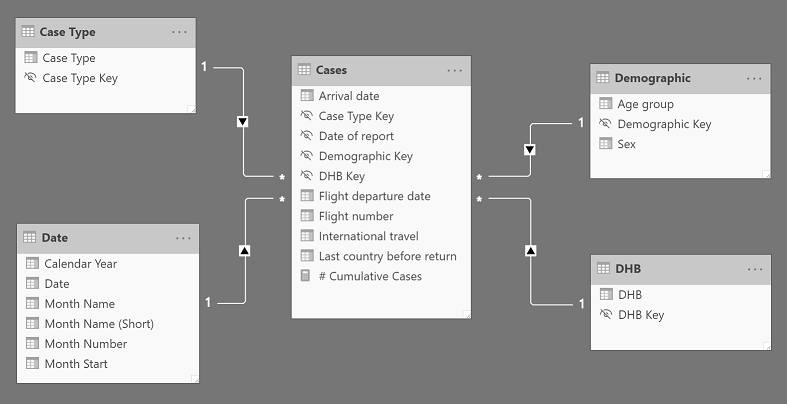
The Excel workbook is pretty easy to pull into Power BI, so I’ve grabbed this as of 6 April 2020 our time and transformed this into a simple star schema of our total cases to date, including a simple measure for # cumulative cases:

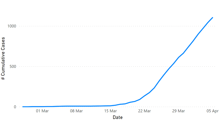
I can then plot # Cumulative Cases on a line chart:

I might want to then explore this further, perhaps by geography. Our data is segmented into District Health Boards (DHBs), so I could add the DHB to the chart as the Legend…

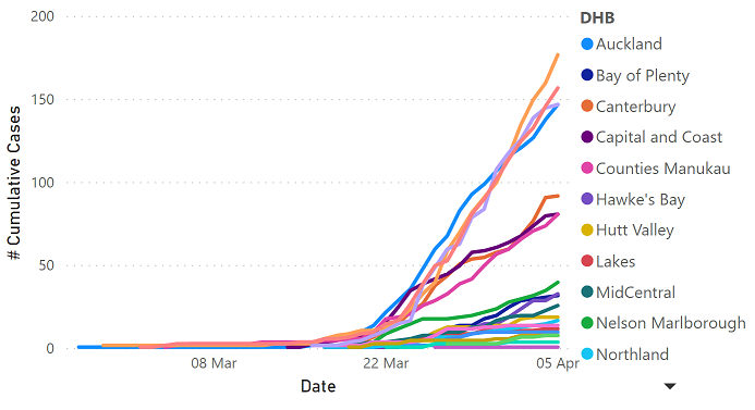
Ouch. We can see the breakdown, but it’s standing room only! There’s also several DHBs that don’t fit on the legend and this, in conjunction with the many series, makes it hard for the reader to derive insights easily. We want our readers to derive insights easily 😊

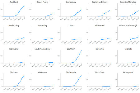
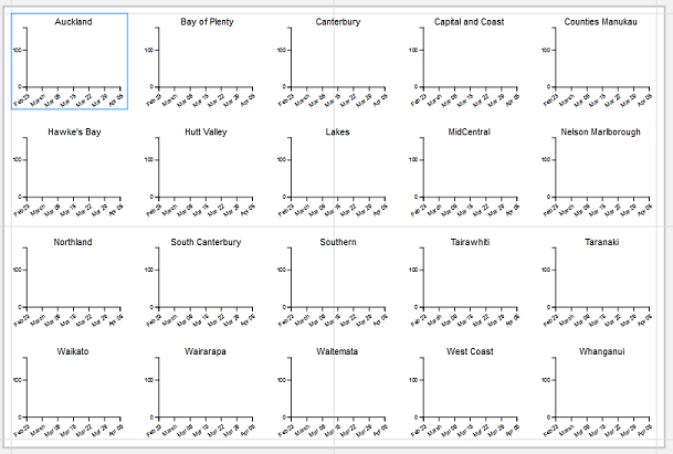
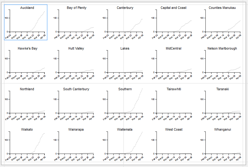
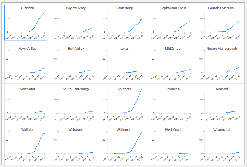
What would be great, is if we could project this into lots of little charts, like so:

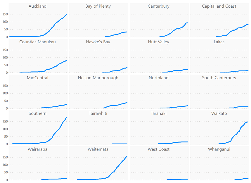
There are currently 20 DHBs in New Zealand - each value of DHB becomes a category, which in turn produces a chart with the same ranges (Date) and values (# Cumulative Cases) for their axes.

Without spending a huge amount of time staring at it, we can easily see that some DHBs started reporting cases quite a way before others, and some currently have a much slower rate of growth than others.

How Can I Make these Myself?

If you’re learning this all for the first time, you might be wondering how to do this in Power BI. At this time, small multiples are not a part of the tooling and - if using the core visuals - the maker will need to craft them manually:

• Create a chart with a filter on the category you want to treat as a small multiple
• Copy/paste filter as many as you need
• Manually set the x/y axis start/end values as appropriate for your data

This is repetitive - and like anything that needs to be done manually - will need to be reviewed to ensure everything is consistent between visuals.

You’ll also need to ensure that you continually update the axis values as things change, as well as manage any new values that might emerge for the category you’re using as a small multiple. More dynamic elements of reporting, such as responding to slicers, also become challenging to incorporate.

The above challenges were actually a catalyst for me to learn the custom visuals framework and produce one of my own. This is a somewhat extreme solution, and not everyone has this amount of patience or time on their hands.

There are many other great custom visuals in the marketplace that provide small multiples as a capability:

• Zebra BI Charts
• Infographic Designer
• Craydec Regression Chart
• 3AG Systems - Column Chart With Small Multiples
• Visuals by Klaus Birringer:
  • Ultimate KPI Card
  • Ultimate Stacked
  • Ultimate Variance
  • Ultimate Waterfall
• Visuals by Akvelon:
  • 100% Stacked Bar Chart
  • 100% Stacked Column Chart
  • Clustered Bar Chart
  • Small Multiple Line Chart
  • Stacked Column Chart

Additionally, you can also use the core R and Python visuals to produce small multiples using their libraries.

The No-Code Alternative

If you haven’t found a custom visual that suits your needs, and you’re not looking to upskill into R or Python right now, you can also give Charticulator a try. This is a tool from Microsoft Research that is primarily designed to create bespoke visual layouts for the web. While Power BI is not its primary target, the tool also has a utility to export designs as a Power BI custom visual.

The team at PowerBI.Tips have also made the tool available on their website. They’ve just introduced the awesome Nested Charts functionality, which I guess is yet another way to describe small multiples! We’re going to use this so that we can produce our very own no-code Power BI small line chart custom visual for the example above.

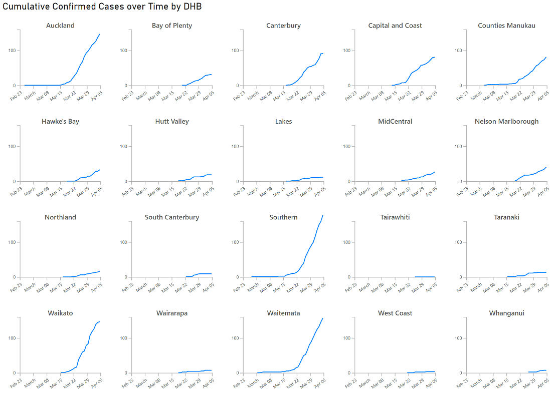
What follows is my preferred way of putting this together. You may have your own requirements and the awesome part of this is how you might apply your own creativity to your own version of this - I would encourage you to do this as soon as you get the hang of things. Here’s my finished product:

I’ve provided the assets from this tutorial at the bottom of the article if you want to skip ahead and audition the finished product before getting into things.

A couple of things to bear in mind:

• Charticulator is an external tool designed for bespoke layouts and as such is not as responsive as core Power BI visuals might be.
• Sometimes a design may not work perfectly inside Power BI, so some experimentation and refinement may be required.
• If your data changes, such as the scenarios above where date and measures may expand, nested charts don’t currently auto-adjust.
• In these cases you will need to modify your visual configuration, re-export and re-import.

Walkthrough

Accessing the Tool

You can do one of the following:

• From the PowerBI.Tips home page, selecting NO CODE - CUSTOM VISUALS from the TOOLS menu.
• Going directly to charts.powerbi.tips

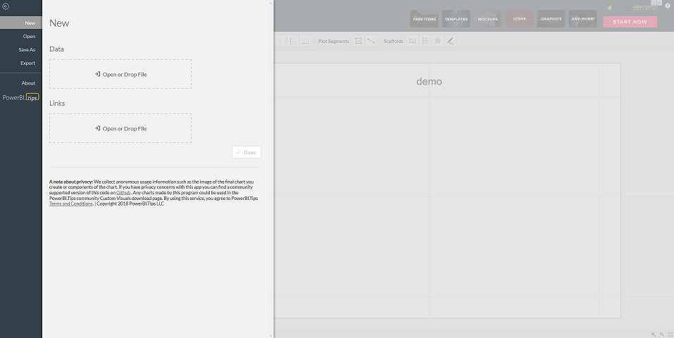
You’ll be greeted with the main screen, e.g.:

Prepping Data for the Visual

The tool requires you to load a comma-separated values (CSV) representation of the data you wish to work with. I can do this by going into my Power BI model and creating a table visual with the 3 fields I want:

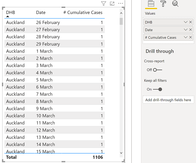
I can then export this by selecting the ellipsis (…) in the visual header and then Export data.

Loading our Data

We then load our CSV data into the tool. Once we do this and click Done, the main canvas will be displayed, e.g.:

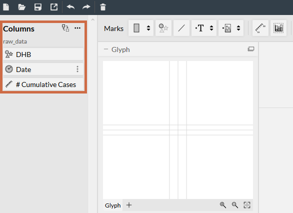
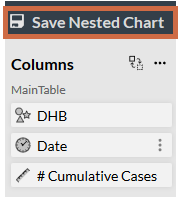
With the canvas available, we should see our fields in the Columns area of the screen - also know as the Dataset Panel, e.g.:

Clearing the Canvas

We want to make as much space available for the visual as possible, e.g.:

What we did above was:

• Delete the auto-generated title by clicking on it and pressing [Delete].
• Drag the visual guides to reduce the amount of whitespace around the edges.

Adding our Mark

Charticulator uses glyphs to represent a row of data. We can add multiple marks to a glyph, so we’ll add the Nested Chart mark to the Glyph editor:

This is a bit hectic! The reason for this is that the tool works a little differently to Power BI: Power BI will aggregate your data down to unique values for each category, whereas the tool will show a glyph for every row of the loaded data, irrespective of whether values are the same or not. We’ll fix this next.

Grouping our Data

We need to make sure that we show one nested chart for each value of DHB instead:

This looks a bit more manageable! What we did above was:

• Clicked the plot segment in the Layers panel.
• Changed its Group By… attribute to DHB.

Accessing the Nested Chart

Now we have laid out our main chart how we want it, we need to access the Nested Chart:

We did this by:

• Clicking on the nested chart in the Layers panel.
• Clicking Edit Nested Chart… in the Attributes panel.

This will open a second instance of Charticulator in a new tab in your browser. This should look almost the same as your other tab, except for the presence of a new button above the Columns panel:

This is where we’ll edit our nested chart.

First-Time Nested Chart Behaviour

There’s currently a bug with the nested chart upon when it’s first opened, the layout isn’t correct. This will sync up correctly if you do anything inside the designer to make a change. I typically drag one of the canvas guides a small amount to refresh the display, e.g.:

Once we do that, our canvas will update to match what we saw from the main chart earlier on.

The nested chart tends to be smaller than a full chart, so I also zoom the canvas in a bit.

Small Multiple Heading

We want our reader to know which category they are viewing the chart for, so we’ll update the chart title, e.g.:

What we did here was:

• Clicked on the title in the Layers panel (we could also click on it in the canvas)
• Dragged the DHB column to the Test field in the Attributes panel

You should notice that the title has been updated to match the name of the first value from the group.

Checking your Changes in the Main Chart

Any time we want to see how the main chart is looking, we can first click the Save Nested Chart button in the top-left corner, and navigate back to the browser tab containing the main chart, e.g.:

We can now see that the change we made above - to update the chart title - works for each instance of the Nested Chart 👍

Adding Axes

Back in the Nested Chart, we’ll add our Date field as the x-axis:

What we did here was:

• Dragged the Date field to the plot segment’s x-axis
• Modified the font sizing by clicking the plot segment, and clicking the ellipsis (…) under X Axis in the Attributes panel
• Dragged the guides to give us the best fit for the font size and Nested Chart canvas

We’ll leave the date format as-is for now; this can be an exercise for you to do once we’ve got the chart working how we want it.

Now, we’ll set up the y-axis with our # Cumulative Cases:

What we did here was:

• Dragged the # Cumulative Cases field to the plot segment’s y-axis
• Modified the font sizing by clicking the plot segment, and clicking the ellipsis (…) under Y Axis in the Attributes panel
• Dragged the guides to give us the best fit for the font size and Nested Chart canvas
• Made any necessary adjustments to the x-axis and Nested Chart guides to maximise space for the data later on

It’s tempting to have a peek at the main chart by saving the Nested Chart and navigating back. I recommend doing this a lot, to make sure things are progressing as you intend. Here’s the whole chart now:

Adding Data Points

Now our axes are all good, we can add our data.

As mentioned above, a glyph represents each row of our data. In a Nested Chart, this is filtered down to the rows that match the grouped value.

To create a line chart, we need to do two key things:

1. Create a mark for the glyph
2. Create links for to connect them together

Let’s start with the mark:

What we did here was:

• Dragged a symbol to the Glyph canvas
• Changed its Size to a smaller number in the Attributes panel

Because the glyph represents each data point and we’ve added our axes, each mark is resolved to its correct x/y coordinates.

To connect the glyphs, we make use of the Links tool, with the default options e.g.:

We’ll save and taken another quick peek at the main chart, now that we have something that shows our data:

We’ve now got the crux of our visual in-place 😊

Cosmetic Improvements

As my intended destination is Power BI and I’m pretty happy with my layout, I’m going to make some cosmetic changes to the Nested Chart, just to make it look a bit more at home.

Small Multiple Heading

What we did here was:

• Selected the title from the Layers panel
• Changed the Font to Segoe UI Semibold (note that while there is a font picker, it’s quite limited, and you can manually type in the name of a known font on your system)
• Changed the Color to something a little less subtle than black. In this case I’ve used one of the Power BI theme defaults: #605e5c

Axes

What we did here for each axis was:

• Selected the plot segment from the Layers panel
• In the Attributes panel, under the axis, clicked the ellipsis (…)
• Modified the Line Color to a lighter shade of grey- I’ve used #bdbdbd from the Power BI default theme
• Modified the Tick Color to match that of the title: #605e5c
• Modified the Font Family to Segoe UI

Glyph Symbol

As like all creations, this is entirely based on personal preference. I want to hide the symbol representing the data points so that I just have the line provided by the links; we still need the symbol in our chart to ensure they get connected together.

What we did here was:

• Clicked the symbol in the Layers panel
• Changed its Fill to (none) in the Attributes panel

Links

Finally, we’re going to make our line stand out a bit more:

What we did here was:

• Clicked the link in the Layers panel
• Modified the Color in the Attributes panel - in this case, I’ve chosen the primary theme colour from the Power BI default theme: #118dff
• Modified the Width in the Attributes panel to make the line slightly thicker
• Dragged the link in the Layers panel to be drawn after the plot segment, meaning that it gets put on top

Final Tweaks to Main Chart

I think we’re now ready to take another look at our main chart, so we’ll save the nested chart and navigate back:

That looks about right!

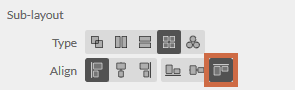
I’m going to make one final change, which may not be evident from this view - if we decide to slice our visual once we’re in Power BI it may not organise correctly, so click the plot segment and set the vertical align to Top in the Attributes panel:

Getting Our Visual into Power BI

We’re now at a point where we can try our visual in Power BI.

Safety First!

Once you’ve loaded into Power BI, you might want to make further tweaks and try again, so before we plough on ahead, it’s a good idea to make sure you’ve saved your chart if you haven’t already. Note that saving your chart will keep it in your browser’s session and this does not guarantee permanent storage. If you want to truly keep your chart for future revisions, you can get it as a .chart file by doing the following:

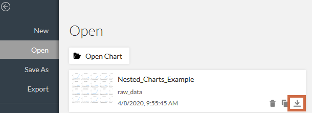
• After saving your chart, click on the Open button in the toolbar
• Find your chart in the list, and click the Download button:

What’s really cool about the PowerBI.Tips tool is that if you’re too excited to get to the Power BI part and forget to do this and export the visual as below, they automatically save the state of your chart at point of export for you in the list 👏

Doing the Export

• From the toolbar, click the Export button
• Select Power BI Custom Visual
• Under the Power BI Custom Visual Properties section, fill in your details as needed, e.g.:

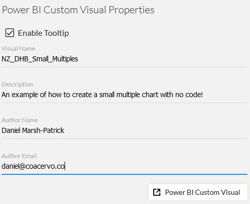
• Click the Power BI Custom Visual button. This will export a .pbiviz (custom visual) file iand you can save this to your machine.

Importing the Custom Visual

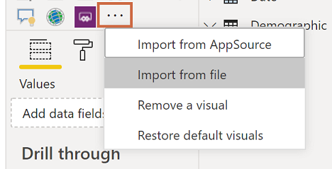
• In Power BI Desktop, click the ellipsis (…) in the Visualizations panel and select Import from file:

• If you’re happy to proceed, confirm you wish to import
• In the dialog, locate your exported file and select Open (or double-click)
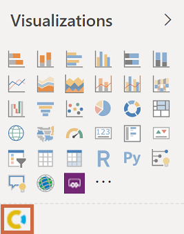
• If you see this in your panel, the visual will now be available to use:

• Click on the visual to add it to your report canvas

Adding Data Roles

If you’ve used the tool you may already have experienced this, but for those who havent, visuals created by charticulator need to work at the same data grain you designed them with in the tool.

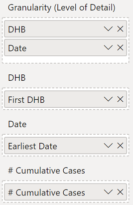
Because our grain is one row per DHB per Date, we need to add both of these fields to the Granularity (Level of Detail) data role to ensure that our glyphs are resolved the same way. We’ll then add our other fields and measures to the other data roled as normal. Mine looks like this:

And… presto!

Assets and Materials

The above was quite a read! I’m hoping that if you’ve reached this you either want to compare your results to mine, or just have a look at the finished product before you start.

Here’s copies of my work for this tutorial:

• Charticulator definition (.chart file)
• Power BI custom visual (.pbiviz file)
• Power BI workbook - containing sample data and the custom visual already loaded

I hope that you’ve found this useful and it gives you some ideas on how to start creating your own no-code custom visuals ith small multiples. Good luck, and have fun!

DM-P